A Calibration Management Specialist's Guide to Type-A Measurement Uncertainties.
1. Introduction.
When we take a measurement, and then state the uncertainty that is associated with our measurement, we are not saying that the quantity we are attempting measure has no single, definite value, we are simply accepting a fact of life that no measuring device has the ability to produce a perfect result.
We are, in fact, reporting, in mathematical terms, how confident we are of our measurement of that quantity. Consider the examples below, they are not supposed to be measurements, they are what is actually happening in the real world. They are statements of fact.
| The current flowing through a resistance is 16.73mA | |
| The length of a steel bar is 1.765 metres | |
| The mass of water in a container is 27kg | |
| The temperature in a room is 25.2 degrees Celsius |
When we try to measure these quantities, we have no way of knowing the real value (the fact). The best that we can do is to use the most accurate equipment we have to produce our interpretation of the value, and then state how accurate we think that our interpretation is.
So, for example, we would report our assesment of the above quantities as follows:
| The current flowing through a resistance was measured as being between 16.72mA and 16.74mA | |
| The length of a steel bar was measured as 1.76 metres to within +/- 0.01 metres | |
| The mass of water in a container was measured as 27kg +/- 2% | |
| The temperature in a room was measured as between 25.15 and 25.3 degrees Celsius |
|
| |
| The Measurand | This is the actual value of the quantity we are attempting measure. |
| The Observed Value | The value that we measure as our interpretation of the measurand. |
| Measurement Error | This is the difference between the Observed Value and the Measurand. |
When we talk about a "Measurement Error" we do not include things such as:
| Misreading of instruments such as analogue gauges | |
| Failure to apply known correction factors to raw data | |
| Incorrect recording or misinterpretation of experimental data |
These are simply mistakes that must be avoided.
In order for any uncertainty analysis to be of use, it is vital to be totally honest. There is nothing to be gained in reporting an uncertainty that is an over-optimistic view of reality, that helps no-one. If an uncertainty appears high, but is derived accurately, this is no imputation of either the equipment or the operator.
What does result from truthful analysis, however, is that the major contributors to the uncertainty are revealed. This information can very often lead to clues on how to refine methods and procedures in order to ensure that each contribution to the total uncertainty is minimised.
2. Repeatability and Uncertainty.
If a measurement is subject to random, and hence unpredicatable, influences there will always be a degree of uncertainty in that measurement. This will reveal itself if repeated observations of the same measurand are all different. The stronger the influence of random factors, the less repeatable our observations will become. By their very nature we cannot correct for them, we can only attempt to quantify how strong their influence is.
If, on the other hand, our observations are subject to non-random, and hence predictable, influences, our readings will at least be repeatable. Furthermore we can correct for their effects, for example:
Example 1 Thermometer:
If for some unknown reason a thermometer always under-reads by 0.2C, this can be added to the indicated value as an offset. Great care must always be taken though to ensure that the offset does not possess any form of drift or randomicity.
Example 2 Magnetic Compass:
A compass always points to Magnetic North, whereas maps refer True North. The difference between the two is called Magnetic Variation, it is a non-random, known quantity. A navigator can therefore correct for variation, and accurately plot his course between two points.
From this we can conclude the following, very important, points:
|
| |
| If a measurement is unrepeatable, there will be an uncertainty associated with that measurement. | |
| If a measurement is unrepeatable, there will be an uncertainty associated with that measurement. | |
|
Non-random influences do not, by themselves, produce measurement uncertainties.
or, put another way: Repeat observations of the same measurand are not subject to measurement uncertainties if the measurement error is constant. . |
|
3. Mean Value and Standard Uncertainty.
If we make repeat observations of the same measurand and each observation yields a different result, we need to find a method of expressing our conclusions as to the value of the measurand, and how our conclusion relates to the spread of the observed values.
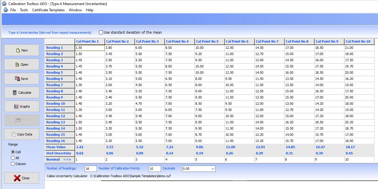
Shown below are a set of repeat observations of a number of calibration points, very much like those which would be produced in many calibration procedures. The measurements are shown in the Calibration Toolbox ADO Type-A Uncertainty Calculator.

The above picture illustrates some key points:
|
| |
| Nominal Value |
Each observation must have a nominal, or reference value.
This could, for example, be the calibrated dimension of a gauge-block, or a temperature indicated by a UKAS calibrated thermometer. In each case, this value must be known to at least an order of magnitude higher that the accuracy required of the observations. |
| The Observed Data |
The data must be genuine repeat observations
For example in the case of a thermometer calibration, it is not acceptable to leave the thermometer in the temperature bath and record the value every minute or so, you must remove the device, wait, replace it, and then wait again for stability, and then make the observation. For a micrometer, the device must be closed onto the gauge block, a measurement recorded, and the jaws re-opened, before repeating the procedure. |
| Spread of Data | As the unrepeatability of the observations increases, so does the number of repetitions required to produce a meaningful sample. |
In the picture, the results calculated by the Uncertainty Calculator can be seen to be:
- The Mean Value
- The Standard Uncertainty
- The Nominal Value
and also shown is:
The Mean Value is the simple arithmetic average of the repeat observations for each calibration point.
The Standard Uncertainty is the internationally accepted method of expressing the dispersion of the observed data about the Mean Value. For the mathematically minded, it is the standard deviation of the observations from the Mean Value. The important thing to grasp though, is that:
The greater the value of the Standard Uncertainty, the less repeatable the observations were, and, of course, vice-versa.
4. Coverage Factor and Expanded Uncertainty
.
Statistical analysis (which is beyond the scope of this article) can show us that, in a properly carried out repeat measurement:
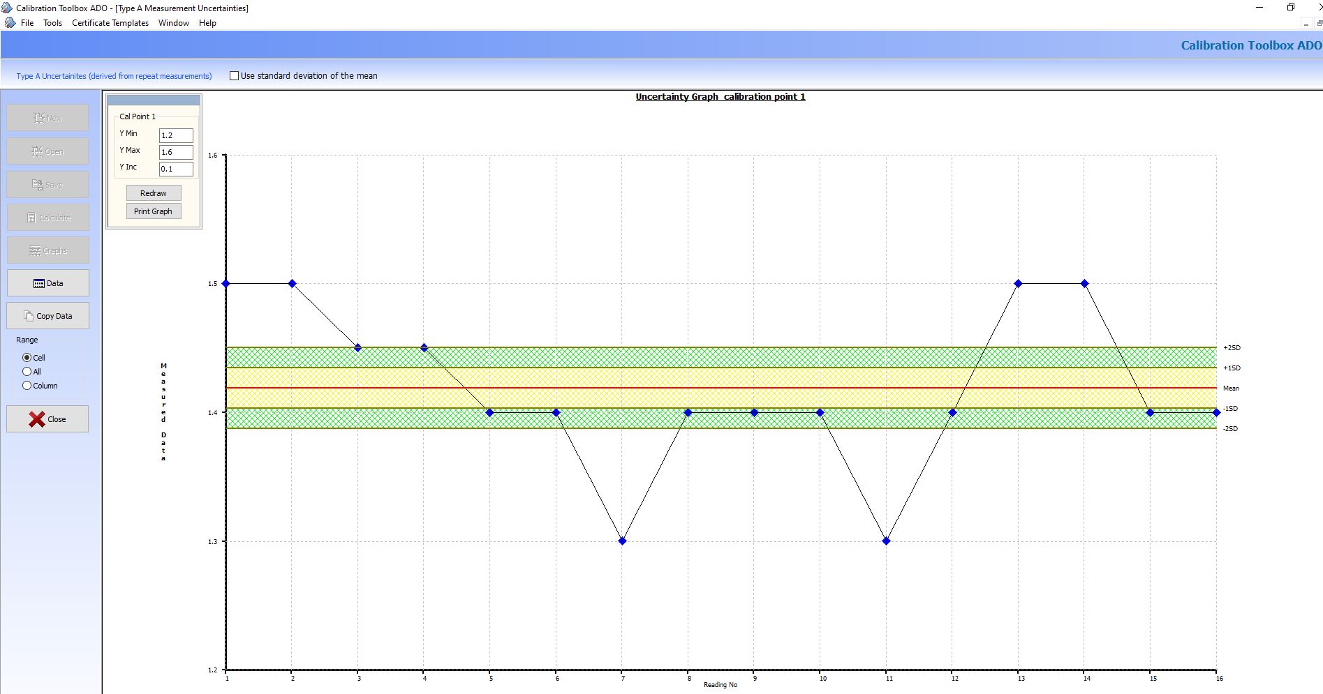
Approximately 68% of the observations will lie in the range:
|
Approximately 68% of the observations will lie in the range:
Mean Value +/- (1 x Standard Uncertainty) |
|
|
Approximately 95% of the observations will lie in the range
Mean Value +/- (2 x Standard Uncertainty) |
The values by which the Standard Uncertainties are multiplied are called Coverage Factors and in calibration work normally have the values of 1 and 2.
The picture below shows the graphical output from the Calibration Tpplbox ADO Uncertainty Calculator, using the first calibration point in the previous example.

5. Useful Links
Here are some links that you might find informative:
NIST: Guidelines for Evaluating and Expressing the Uncertainty of NIST Measurement Results
